Regression Analysis

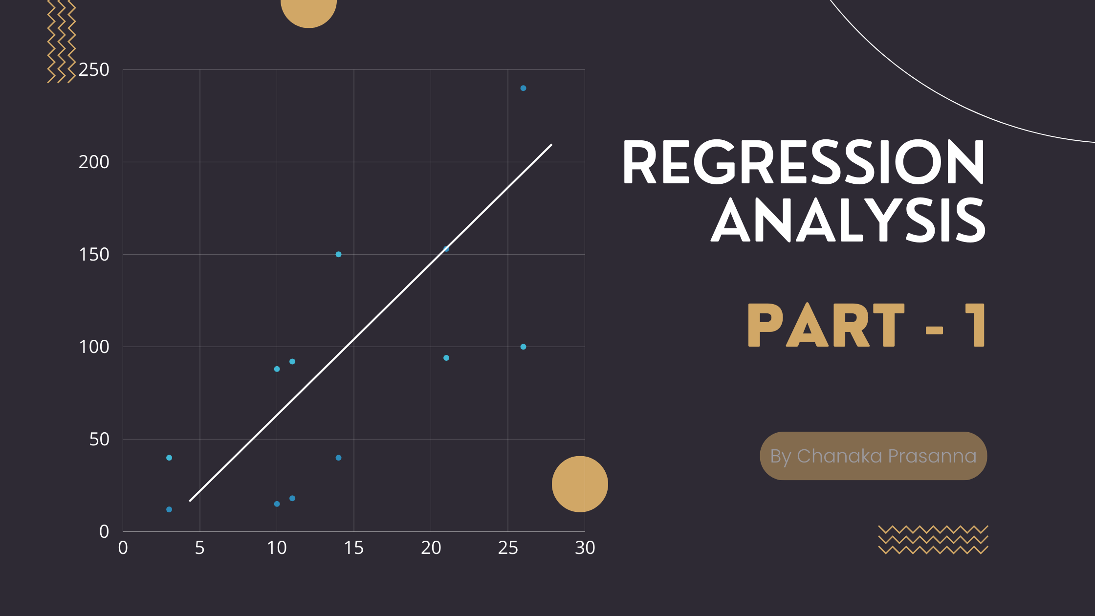
When dealing with data in the real world, you may encounter some variables (features) that have some relationships between them. These relationships may be linear or nonlinear. So, regression analysis is a technique used to find/model relationships between variables.

For example, How do students' marks on the statistics module vary based on study time? To find out this, we need regression analysis.

In the regression analysis, we have three forms:

• Simple Linear Regression - When we have one independent variable. The Dependent variable is a metric
  • Ex:- Exam results based on the study time
• Multiple Linear Regression - When we have more than one independent variable. The Dependent variable is a metric

Ex:- Exam results based on study time, mobile phone usage, sleep time

• Logistic Regression - When we have categoricalvariables. The Dependent variable is a metric
  • Ex:- Predicting whether a student will pass or fail an exam based on their study time, mobile phone usage, and sleep time (where the outcome is pass/fail rather than a continuous score).

Here all independent variables can be either metric, ordinal, or nominal from all forms of regression analysis.

Here we will discuss about the simple linear regression model.

Simple Linear Regression Model

The simplest regression model includes two variables (x—independent variable, y—dependent variable).

As we know, the equation for two variables scenario to denote a linear relationship is y = mx + c . But in statistics, normally we use different symbols to denote m (Slope) and c (Intercept). Here we use ŷ instead of y since it is the predicted value. Not true value.

New version with new symbols

ŷ_i = β₀ + β₁ x_i

Where:

• (ŷ_i ) is the i^th predicted value (value of dependent variable).
• (x_i ) is the i^th input feature (value of independent variable).
• (β₀) is the intercept (constant term).
• (β₁) is the coefficient (slope) for the feature (x_i ).

Hey, Do you know how I drew this red line? Is this the best representation of all data points?

You can draw many linear models with the dataset. If so, how do you choose the best model?

Model - Mathematical representation of a system or Approximation of the reality

Well, we need to find a model ( think of it as a one-line in Figure 1.1 ) that minimizes the error term.

So what is meant by error here? Look at this image below. ε represent error. In other words, the difference between the true y value and predicted y value.

So the true value can be represented as

y_i = ŷ_i + ε_i

ŷ_i = β₀ + β₁ x_i

y_i = β₀ + β₁ x_i + ε_i

Where:

• ε_i is the error for given x_i and predicted y_i

If the true value of y is on the regression line, the error is 0 for a given x value.

One important thing is to note that, there are two ways to find solutions for regression models.

1. Analytical method (Closed-form solution)

• Possible for a limited number of use-cases - Ex:- When we have a huge number of variables in the model, it's difficult for humans to solve

2. Approximate iterative solution (Numerical solution)

• Iterative process. It gives an approximated value as a solution

First, let's see how we can apply the analytical method for the simplest regression model

Finding the best linear regression model for a given dataset using the analytical method

Linear Regression Model

y_i = β₀ + β₁ x_i + ε_i

Cost Function [Sum of Squared Errors - S(β0, β1) ]

S(β₀,β₁) = Σ (y_i - (β₀ + β₁ x_i))²

If we consider the sum of errors, it will be approximately zero. So we have to consider the squared sum of error.

It is a function of beta_zero and beta_one

Taking Partial Derivatives

Partial Derivative with respect to β0 

∂(S)/∂(β₀) = -2 Σ (y_i - (β₀ + β₁ x_i))

Partial Derivative with respect to β1 

∂(S)/∂(β₁) = -2 Σ (y_i - (β₀ + β₁ x_i)) x_i

Setting the Partial Derivatives to Zero

To minimize the cost function, we set these partial derivatives equal to zero because, at the minimum or maximum points, the derivative is equal to zero.

For β₀:

Σ (y_i - (β₀ + β₁ x_i)) = 0 --------> 1
n β₀ + β₁ Σ x_i = Σ y_i

For β₁:

Σ (y_i - (β₀ + β₁ x_i)) x_i = 0 --------> 2
β₀ Σ x_i + β₁ Σ x_i² = Σ x_i y_i

Solving the System of Equations

Rearranging the equation

β₀ = (Σ y_i - β₁ Σ x_i) / n

β₀ = (Σ y_i) / n - (β₁ Σ x_i )/ n

β₀ = ŷ - β₁ x̄ --------> 3

Substitute this into the second equation to solve for β1

(ŷ - β₁ x̄) Σ x_i + β₁ Σ x_i² = Σ x_i y_i

since Σ x_i = n x̄

nx̄ŷ - nβ₁ x̄² + β₁ Σ x_i² = Σ x_i y_i

β₁ = (Σ x_i y_i - nx̄ŷ) / (Σ x_i² - nx̄²) --------> 4

3 and 4 equations give us the exact solutions for β0 and β1.

Now, since we know the β0 and β1 we can find the regression model.

Finding the best linear regression model for a given dataset using the numerical analysis

Our cost function is: (Sum of squared errors)

S(β₀, β₁) = (1/2n) * Σ (y_i - (β₀ + β₁ x_i))²

where:

• n - number of data points

Now the goal is to minimize the error represented using the equation S(β0, β1) based on the β0 and β1 . We’re using 1/n​ in the equation to average the total error. Instead of summing the squared errors directly (which could get huge if we have a lot of data), we divide by n to get the average error per sample. This way, no matter how many data points you have, you get a normalized error that’s easy to work with. Since we are finding the value of β0 and β1 when the function reaches its minimum, there is no problem to use 1/2 in the equation to simplify the calculations. Let's clarify it below.

In the 1.4 image, the value of x at minimum is zero.

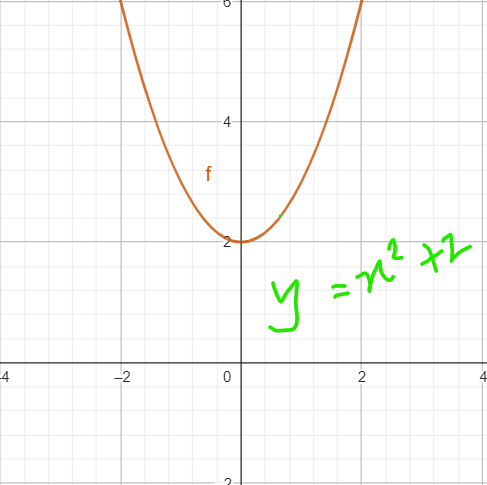
After multiplying the equation by 0.5

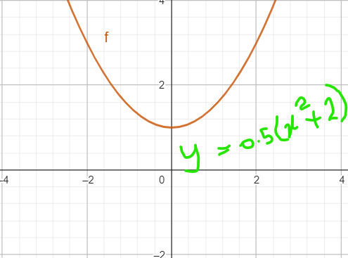
You can see, still the value of x at minimum is zero.

Okay, Let's continue from where we left.

Now we need to find the best β0 and β1 that give the minimum error. That means we are having an optimization problem.

S(β₀, β₁) = (1/2n) * Σ (y_i - (β₀ + β₁ x_i))²

You can see that this function is non-linear. Also, it has more than one variable ( β0 and β1 ) leading to call it a multidimensional equation.

To find optimized values of a non-linear multi-dimensional equation, we have methods:

• Gradient-based method
  • The function should be differentiable and continues
  • Examples
    • Gradient Descent Algorithm Variants
      • Batch Gradient Descent
      • Stochastic Gradient Descent
      • Mini Batch Gradient
    • Hessian Based Algorithms
      • Newton Method
      • Quasi-Newton Method
• Non-gradient Based Algorithms
  • For non-differentiable functions
  • Examples
• Golden Section Search
• Nelder Mead

In this section, we will focus exclusively on the Gradient Descent Algorithm.

The gradient descent algorithm is a first-order iterative optimization algorithm for finding the local minimum of a differentiable function. I hope you know that gradient refers to the slope of a given point.

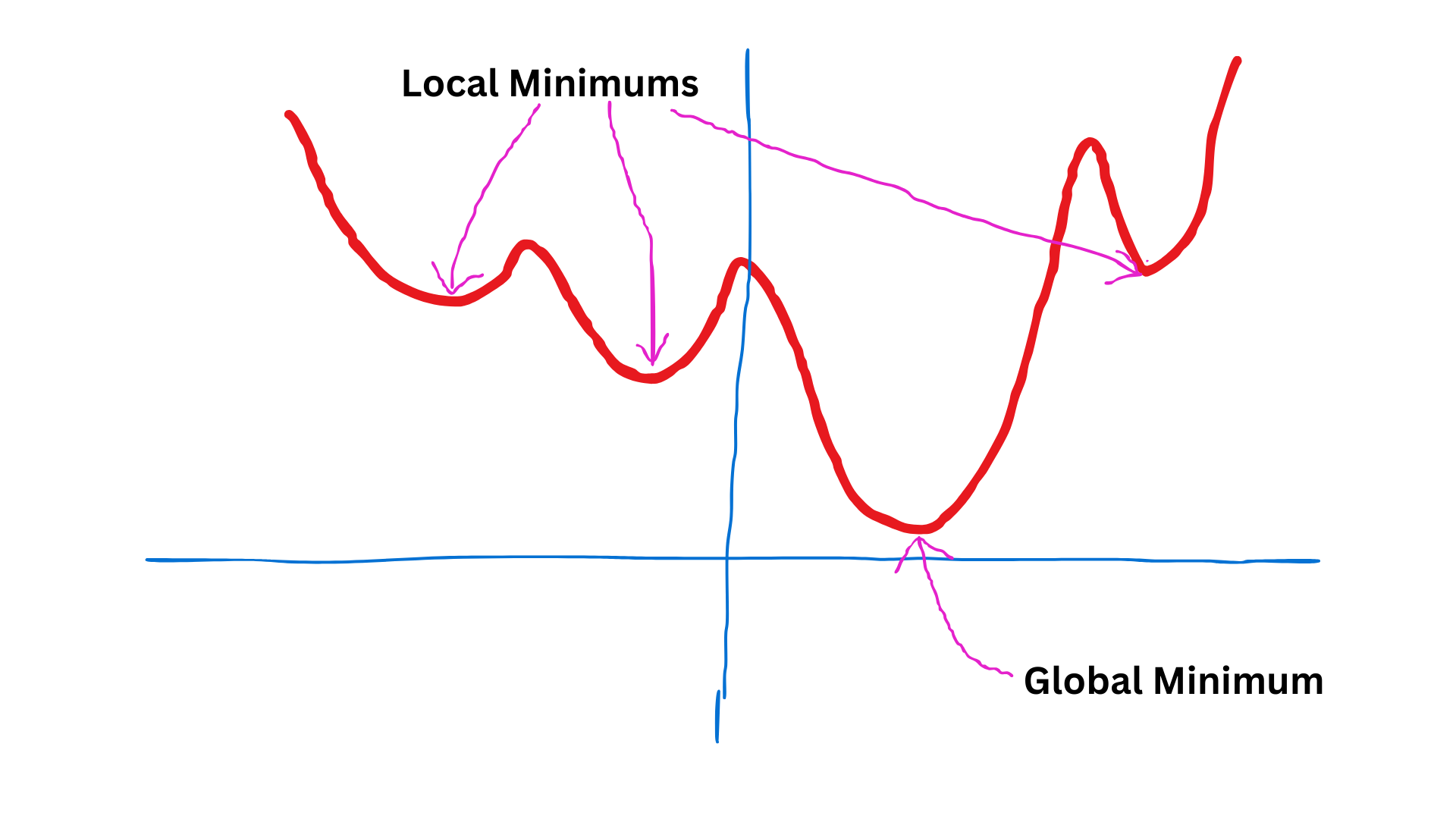
Basic steps to follow in this process when finding the best β0 and β1the .

1. Starts with some values for β0 and β1 .
2. Pick the next point

xⁿ⁺¹ = xⁿ + αⁿ * ∇S(β₀, β₁)

Where:

• ∇S(β₀, β₁) = partial derivatives of S based on β₀ and β₁
• xⁿ⁺¹ = x value of the next point
• xⁿ = x value of the current point
• αⁿ = learning rate

Above equation is general one. Let's consider it with β₀ and β₁.

β_{0_next} = β_{0_current} + αⁿ * ∂S(β₀, β₁) / ∂β₀

β_{1_next} = β_{1_current} + αⁿ * ∂S(β₀, β₁) / ∂β₁

This process happens simultaniously

This image shows the convergence towards the minimum

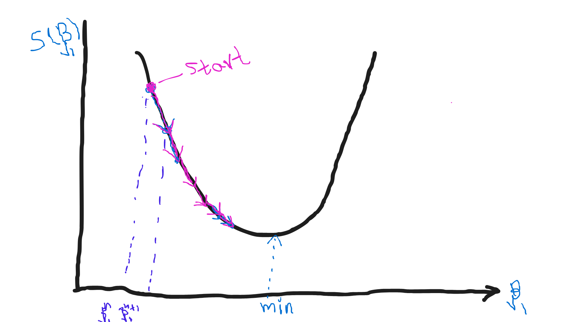
If the gradient is greater than zero, we are on the right to the minimum. That means convergence happens from the right side. If the gradient is less than zero, we are on the left to the minimum. So the convergence will start from the left side as shown in 1.7 image.

For each iteration, we have to find a new best α as well. That process is also an optimization problem.

Let's consider equation for next point:

xⁿ⁺¹ = xⁿ + αⁿ * ∇S(β₀, β₁)

Let's assume,the starting point (where n=0), xⁿ = p⁰ and ∇S(β₀, β₁) = S₀, xⁿ⁺¹ = p¹. Note that, in each iteration, first we need to find normalized gradients for each point.

So the equation is: p¹ = p⁰ + α⁰S₀

Also we know y = β₀ + β₁ x = f(x), f(x) is nothing but function of x

Since we know the equation for the point p¹, we can take function value as f(p¹). Not that, the p¹ is the x value of next point.

f(x) = β₀ + β₁ x
f(p¹) = p⁰ + α⁰S₀
So, f(p¹) = β₀ + β₁ * ( p⁰ + α⁰S₀)

Here the only variable is α⁰. Eventhough we are finding the β₀ and β₁, finding the best α happens for given β₀ and β₁ . So it's a linear function of α.

So we can find the best α⁰ by optimizing this linear function. For the optimization process, we need to usenon-linear optimization methods like golden section search. Sometimes, depending on the initial function you are going to optimize, you may have a non-linear function for α as well. In such cases, you can use any non-linear optimization methods.

Now we know the best value for α⁰ and the next point p¹

3. Repeat the above process for β0 and β1 until β0 and β1 reaches the stopping criteria.

• You may stop the process when the gradients approaches to zero.

After you find the minimum values for β0 and β1 , we can write our best model.

If you remember, during the process we had to find the best α for each iteration. This is a drawback of this method.

Anyway, why the value of α is important?

It's because this defines the step size.

When we choose larger values for α ( image 1.8 ), it overshoots the minimum. If we choose smaller values for α, then it take more time to reach its minimum. That is why we need to find the best α for each iteration. Since this is a limitation in this method, the Newton method is introduced.

In this blog, we explored the basics of simple linear regression, a foundational method in regression analysis. We learned how to build a linear regression model, use the analytical method to derive the best-fit line, and explored the gradient descent algorithm for solving more complex optimization problems. Understanding simple linear regression is crucial because it forms the basis for more advanced techniques.

In the next blog, we will dive deeper into multiple linear regression, where multiple factors influence the outcome, and logistic regression, which is ideal for classifying outcomes. Stay tuned for more insights!