Multiple Linear Regression - Ordinary Least Squares Method Explained
In the realm of data analysis, understanding the relationships between variables is crucial. One of the most powerful tools for uncovering these relationships is regression analysis. While I previously explored the fundamentals of regression and linear regression, this blog post delves deeper into multiple linear regression. This technique allows us to analyze how multiple input features contribute to a single output variable, helping us make predictions and informed decisions based on complex data sets. I’ll explore the mathematical foundations and the least squares estimation method, ultimately providing you with a comprehensive understanding of multiple linear regression.
Link for the previous blog post.
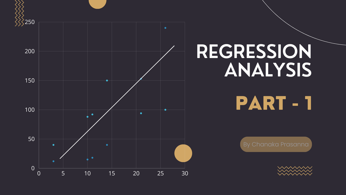
Here we are gonna discuss multiple linear regression in detail. It's clear that we have a linear equation with multiple input features. However, we assume that the model gives a single output.
y = ŷ + ε
Model:
ŷ = w0 + w1x1 + ... + wdxd
where :
- w0 is the bias or intercept
- from w1 to wd are weights or coefficients
- ε is the error
- ŷ is the predicted value
| x1 | x2 | x3 | ... | xd | y |
|---|---|---|---|---|---|
| x11 | x12 | x13 | ... | x1d | y1 |
| x21 | x22 | x23 | ... | x2d | y2 |
| x31 | x32 | x33 | ... | x3d | y3 |
| ... | ... | ... | ... | ... | ... |
| xn1 | xn2 | xn3 | ... | xnd | yn |
Here Xnd represents the nth data point of dth feature.
Now we can represent all the above instances using:
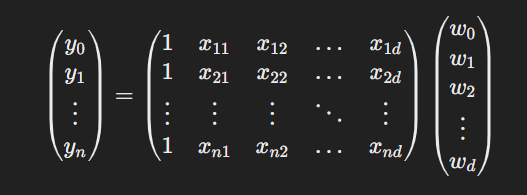
The output vector y is n × 1 vector, X is n × (d+1) matrix and w is (d+1) × 1 vector.
Now the model can be represented as below.
ŷ=Xw
Sometimes, you may confused about the column of 1s in matrix X.
So let's take an example and clarify it first.
Suppose we have a dataset with 2 features (x1 and x2) and 3 instances.
ŷ = w0 + w1x1 + w2x2
| Instance | 𝑥₁ | 𝑥₂ | 𝑦 |
|---|---|---|---|
| 1 | 2 | 3 | 10 |
| 2 | 4 | 5 | 20 |
| 3 | 6 | 7 | 30 |
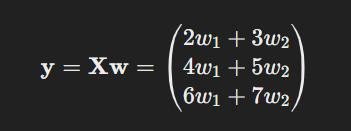
Without Column of 1s
If we exclude the intercept term, the model matrix X and weight vector w would look like this.

So, the output vector Y would be.
With Column of 1s
To include the intercept w0, we modify X and w.
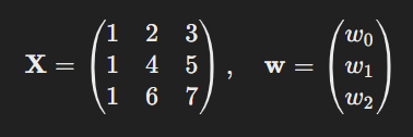
Now, the output vector would be

Now you know the reason to add a column of 1s in X.
Our objective of this problem is to minimize the error.
Least Square Estimation method
In the Least Square Estimation method, we calculate the average of the sum of squared errors.
ε = y - ŷ
ε = y - Xw
Both y and ŷ are n x 1 vectors.
As we know, the y and the inputs are known, and the objective function is a function of w (This includes the weights and bias).
So we can write the objective function as a function of w (bias: w0 + weights: w1 to wd) as:
J(w) = Σε2 / 2n
As we know, Σy2 can be written as:

Then, let's express Y as a matrix

The sum of squares can be rewritten using matrix multiplication, where the transpose of Y, YT, is multiplied by Y:

So we can write Σε2 as εT ε
ε = y - Xw
Then the objective function can be written as:
J(w) = (y-Xw)T (y-Xw) / 2n
J(w) = (yT-wTXT) (y-Xw) / 2n
J(w) = ( yTy - yTXw - wTXTy + wTXT Xw ) / 2n
Since yTXw and wTXTy are the same,
J(w) = ( yTy - 2wTXTy + wTXT Xw ) / 2n
To find the minimum, we need to get derivatives of this function and set it to zero.
∂J(w) / ∂w = 0
∂ [(yTy - 2wTXTy + wTXT Xw) / 2n ] / ∂w = 0
0 - 2XTy +XT Xw = 0
w = (XT X)-1 XTy
Now we have a vector of values for w. This is a closed-form solution where we know exact values. Sometimes we have scenarios in the real world where we can't apply closed-form methods. In that case, we have to use the numerical optimization methods. For this multiple linear regression model also you can follow same steps as I mentioned in previous blog post.
In summary, multiple linear regression is a valuable technique for modeling relationships between several independent variables and a dependent variable. The least squares estimation method provides an efficient way to minimize errors, leading us to optimal weights for our model. While closed-form solutions are beneficial, it's essential to remember that in real-world scenarios, numerical optimization methods may also be necessary. Understanding these concepts will empower you to leverage multiple linear regression in various applications, enabling better predictions and insights from your data.
If you found something useful here, subscribe to me.

