Learning

Let's Compare Different Kernels for SVM Models

Chanaka Prasanna

Aug 28, 2024 • 9 min read

Support Vector Machines (SVMs) are a versatile tool in machine learning, capable of handling both linear and complex non-linear data through the use of kernel functions. Kernels allow SVMs to transform data into higher dimensions, making it easier to find optimal decision boundaries. In this blog post, we will:

Understand Kernels -Learn what kernels are and their role in SVMs.
Explore Kernel Types - Compare different kernel functions—linear, polynomial, RBF, and sigmoid.
Analyze Models - Examine how each kernel performs on the Iris dataset.
Compare Results - Visualize decision boundaries to see how different kernels impact classification.

By the end, you'll have a clearer understanding of how to choose the best kernel function to enhance the performance of your SVM models.

Before you read this blog, I recommend you to go through this article since it covers the basics of SVMs.

Download full notebook here.

Download

SVM Classifiers and Kernels

In this section, we’ll explore the concept of kernels in Support Vector Machines (SVMs) and demonstrate how different types of SVM classifiers behave on the Iris dataset. Specifically, we’ll look at four SVM classifiers, each using a different kernel. But first, let’s understand what a kernel is and why it’s important.

Introduction to Kernels in SVMs

The Kernel functions in SVMs are like clever shortcuts that let the model spot patterns in data more effectively. Instead of working with the original data, kernels transform it into a higher dimension, where it’s easier to separate different groups. This makes SVMs capable of drawing more complex boundaries, which helps in making better predictions. There are different types of kernels—linear, polynomial, RBF, and sigmoid—each suited for different types of data. Choosing the right kernel is key to making sure the SVM not only learns well but also predicts accurately. There are two main types of kernels:

Linear Kernels
- A linear kernel is the simplest form of a kernel. It assumes that the data is linearly separable, meaning a straight line (or hyperplane in higher dimensions) can separate the different classes.
- Use Case --> When the data is already well-separated by a straight line, a linear kernel works best. It is also computationally efficient.
Non-Linear Kernels
- Non-linear kernels, such as the Radial Basis Function (RBF) or Polynomial kernels, can model more complex decision boundaries that are not straight lines. They map the input features into a higher-dimensional space where a linear separator can be found.
- Use Case --> When the data is not linearly separable, non-linear kernels are used to create more flexible and complex decision boundaries.

Follow this video for more details. YT Channel -> Visually Explained

Okay, Let's understand how different kernels work using an example. Here we use the Iris dataset from Scikit-Learn.

# Import necessary tools
import matplotlib.pyplot as plt
from sklearn import datasets, svm
from sklearn.inspection import DecisionBoundaryDisplay

matplotlib.pyplot - Provides functions for creating and customizing plots and visualizations in Python.

sklearn.datasets - Contains functions to load and generate sample datasets for machine learning.

sklearn.svm - Includes tools for Support Vector Machines, a popular method for classification and regression.

sklearn.inspection.DecisionBoundaryDisplay - Visualizes the decision boundaries of classifiers to show how they separate different classes.

iris = datasets.load_iris()

X = iris.data[:, :2]
y = iris.target

iris = datasets.load_iris() - Loads the Iris dataset, which is a classic dataset for classification tasks, containing features and labels for iris flowers.

X = iris.data[:, :2] - Select only the first two features (Sepal length and sepal width) from the dataset for simplicity, as the original dataset has four features.

y = iris.target - Retrieves the target labels (classes) corresponding to the data points in the dataset.

# Check the first 5 records for both X and y
X[:5],y[:5]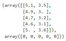

def plot_svm_decision_boundaries(models, titles, X, y, feature_names, figsize=(12, 6)):
    """
    Plots decision boundaries for a list of SVM models.

    Parameters:
    - models: List of trained SVM models
    - titles: List of titles for each subplot
    - X: Feature data
    - y: Target labels
    - feature_names: List of feature names for axis labels
    - figsize: Size of the figure
    """
    num_models = len(models)
    
    # Set up the plot
    fig, sub = plt.subplots(1, num_models, figsize=figsize)
    
    # Ensure sub is iterable even if there's only one subplot
    if num_models == 1:
        sub = [sub]
    
    plt.subplots_adjust(wspace=0.4)

    X0, X1 = X[:, 0], X[:, 1]

    # Plot decision boundaries for each model
    for clf, title, ax in zip(models, titles, sub):
        disp = DecisionBoundaryDisplay.from_estimator(
            clf,
            X,
            response_method="predict",
            cmap=plt.cm.coolwarm,
            alpha=0.8,
            ax=ax,
            xlabel=feature_names[0],
            ylabel=feature_names[1],
        )
        ax.scatter(X0, X1, c=y, cmap=plt.cm.coolwarm, s=20, edgecolors="k")
        ax.set_xticks(())
        ax.set_yticks(())
        ax.set_title(title)

    plt.show()

This function is defined to plot decision boundaries for multiple SVM models at once.

if num_models == 1: sub = [sub]

sub array (or list) represents the individual subplots (graphs) within the figure.
When you create a single subplot using plt.subplots(1, 1), sub is an AxesSubplot object, not a list or array.
The rest of the function assumes that sub is a list, so this line wraps the sub object in a list to make it iterable.
This allows you to use a uniform loop structure later in the function, even if there’s only one subplot.

plt.subplots_adjust(wspace=0.4)

This adjusts the amount of horizontal space (wspace) between subplots. When you have multiple subplots side by side, the default spacing might be too tight, making it difficult to distinguish between them.
By increasing wspace, you create more separation between the subplots, making the plot more readable.

X0, X1 = X[:, 0], X[:, 1]

This separates the two features (columns) from the feature matrix X into X0 and X1.

`response_method="predict"`

It specifies how the model should generate the decision boundary.
"predict" tells the method to use the model's predict function to determine the decision boundary.

cmap=plt.cm.coolwarm

cmap stands for "color map," which determines the colors used to represent different regions in the plot.
plt.cm.coolwarm is a specific color map that transitions from cool colors (like blue) to warm colors (like red).

`alpha=0.8`

Controls the transparency of the decision boundary plot.

`ax=ax`

Specifies the subplot where the decision boundary should be drawn.

ax.scatter(X0, X1, c=y, cmap=plt.cm.coolwarm, s=20, edgecolors="k")

Plots the data points with colors representing classes (y), using the coolwarm color map, point size 20, and black edge color (edgecolors="k").

Before going further, let's understand how zip function works

Given two or more iterables, zip pairs elements from each iterable based on their position.

For example

# Example with two lists
list1 = [1, 2, 3]
list2 = ['a', 'b', 'c']

zipped = zip(list1, list2)
print(list(zipped))  # Output: [(1, 'a'), (2, 'b'), (3, 'c')]

Output --> [(1, 'a'), (2, 'b'), (3, 'c')]

In our case, the zip function combines these lists into tuples

Each tuple contains one model, one title, and one subplot axis.
This allows you to loop through each tuple and unpack its elements into clf, title, and ax.

C = 1.0 # SVM regularization parameter

clf_svc = svm.SVC(kernel="linear", C=C)
clf_svc.fit(X, y)

clf_linear_svc = svm.LinearSVC(C=C, max_iter=10000)
clf_linear_svc.fit(X, y)

clf_rbf = svm.SVC(kernel="rbf", gamma=0.7, C=C)
clf_rbf.fit(X, y)

clf_poly= svm.SVC(kernel="poly", degree=3, gamma="auto", C=C)
clf_poly.fit(X, y)

In this code, you create and train four different Support Vector Machine (SVM) models using the scikit-learn library

The C parameter in SVM controls the trade-off between maximizing the margin and minimizing classification errors. A higher C value penalizes misclassifications more strictly, making the model aim for fewer errors, which can lead to overfitting. Conversely, a lower C value allows more misclassifications, leading to a wider margin and potentially better generalization but with a risk of underfitting.

clf_svc - A standard SVM model with a linear kernel.
clf_linear_svc - A LinearSVC model, which is a faster implementation of an SVM with a linear kernel.
clf_rbf - An SVM model with a Radial Basis Function (RBF) kernel, which is commonly used for non-linear data.
clf_poly - An SVM model with a polynomial kernel of degree 3, useful for capturing polynomial relationships in the data.

The gamma parameter in SVM, specifically for models using the RBF (Radial Basis Function) and polynomial kernels, defines how far the influence of a single training example reaches.

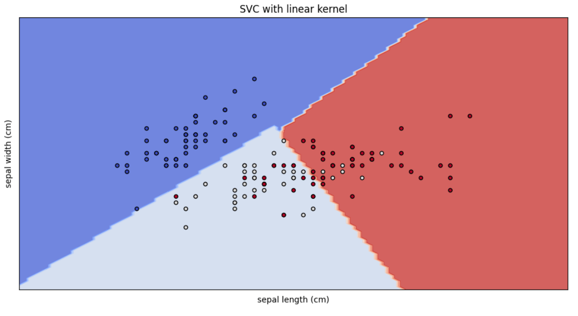
models = [clf_svc]
titles = ["SVC with linear kernel"]

plot_svm_decision_boundaries(models, titles, X, y, iris.feature_names)

Here we are plotting the SVC model with linear kernel.

models = [clf_linear_svc]
titles = ["LinearSVC (linear kernel)"]

plot_svm_decision_boundaries(models, titles, X, y, iris.feature_names)

Now the LinearSVC model.

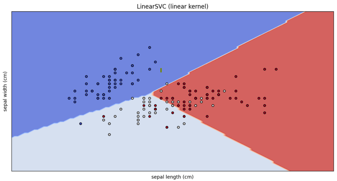
Now you may think, these two models' out puts are same. Actually they aren't. If you look at closely, you can see the difference of decision boundaries. Let's compare those.

# Define models and titles
models = [clf_svc, clf_linear_svc]
titles = ["SVC with linear kernel", "LinearSVC (linear kernel)"]

# Plot decision boundaries
plot_svm_decision_boundaries(models, titles, X, y, iris.feature_names)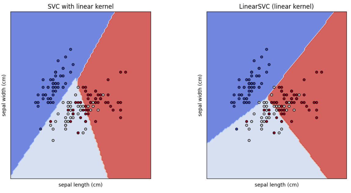

Now you can see the difference.

As per the documentation, The linear models LinearSVC() and SVC(kernel='linear') yield slightly different decision boundaries because,

LinearSVC minimizes the squared hinge loss while SVC minimizes the regular hinge loss. (Refer this link for more information)
LinearSVC uses the One-vs-All (also known as One-vs-Rest) multiclass reduction while SVC uses the One-vs-One multiclass reduction.

Let's understand One-vs-All and One-vs-One.

One-vs-All (One-vs-Rest)

For a classification problem with multiple classes, One-vs-All (OvA) creates one classifier per class.
Each classifier distinguishes one class from all others.

Example :- Imagine you want to classify fruits into three categories. Apple, Banana, and Cherry.

Create Classifiers
- Classifier 1 - Distinguishes Apple vs. Not Apple (Banana, Cherry)
- Classifier 2 - Distinguishes Banana vs. Not Banana (Apple, Cherry)
- Classifier 3 - Distinguishes Cherry vs. Not Cherry (Apple, Banana)
Prediction
- For a new fruit, each classifier gives a score indicating how likely it is to be its class.
- The class with the highest score is chosen as the final prediction.

One-vs-One

For a classification problem with multiple classes, One-vs-One (OvO) creates a classifier for every pair of classes.
Each classifier distinguishes between two classes.

Example :- Again, classifying fruits into Apple, Banana, and Cherry.

Create Classifiers
- Classifier 1 - Distinguishes Apple vs. Banana
- Classifier 2 - Distinguishes Apple vs. Cherry
- Classifier 3 - Distinguishes Banana vs. Cherry
Prediction
- For a new fruit, each classifier provides a vote for one of the two classes it compares.
- The class that receives the most votes across all classifiers is chosen as the final prediction.

I think, Now you know the reasons for difference between SVC model with linear kernel and the LinearSVC model.

models = [clf_poly,clf_rbf]
titles = ["SVC polynomial (degree 3) kernel","SVC rbf kernel"]

# Plot decision boundaries
plot_svm_decision_boundaries(models, titles, X, y, iris.feature_names)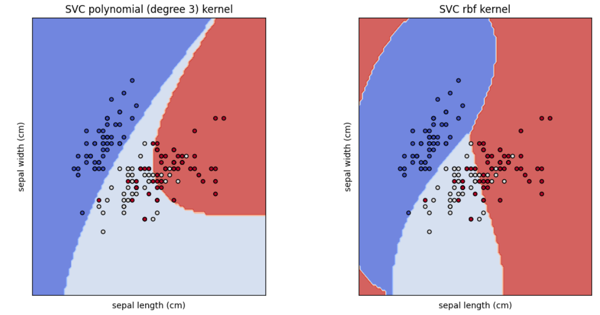

This code section creates, two SVC models with the kernels rbf and polynomial

In summary, kernels are powerful tools in SVMs that help in creating complex decision boundaries by transforming data into higher dimensions. By using different kernels—linear, polynomial, RBF, you can tailor SVMs to handle various types of data and classification challenges. Our exploration with the Iris dataset showed how each kernel affects decision boundaries and classification performance. Choosing the right kernel is crucial for optimizing your SVM model, ensuring it accurately captures the patterns in your data.

If you read up to this point, that means you got something from here. So encourage me to write more like this by subscribing me. And don't forget to follow me on LinkedIn as well. Also, help your friends by sharing this.

SVM Classifiers and Kernels

Introduction to Kernels in SVMs

response_method="predict"

alpha=0.8

ax=ax

One-vs-All (One-vs-Rest)

One-vs-One

Sign up for more like this.

`response_method="predict"`

`alpha=0.8`

`ax=ax`