Identifying the Decision Boundary in Support Vector Machines (SVMs)

In models like regression models, we minimize the error function to get the best-fitting model. However, some problems can occur during the optimization process. The optimal point may depend on the type of loss function or the initial starting point. Sometimes, you might not reach the global minimum. But in SVMs, such problems do not exist. It always has a fixed boundary that separates the classes.

What are support vectors?

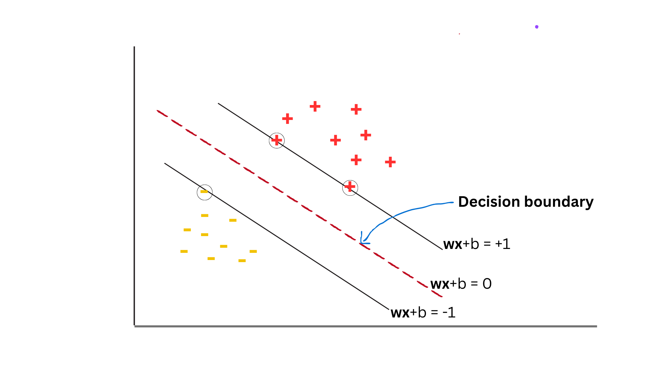
Support vectors are the data points that help to identify the class boundaries in an SVM. In the given picture, there are three support vectors—one from the negative class and two from the positive class. They are highlighted with circles. These support vectors play a crucial role in determining the class boundaries, which in turn define the decision boundary.

Here, we draw a decision boundary in such a way that it has the maximum width separating the positive samples from the negative samples.The decision boundary lies exactly in the middle. For the simplicity of the calculations, we define y = +1 as the desired output of the positive class and the y = -1 as the desired output of the negative class.

Now, we can define the class boundaries as follows:

• For the positive class: w^Tx+b = +1
• For the negative class: w^Tx+b = -1

Where:

• w: Weight vector
• x: Feature vector
• b: Bias

Any point that satisfies the above two conditions we can consider as support vectors. In the middle of theclass boundaries, we have the decision boundary: w^Tx+b = 0.

• For any data point in the positive class (y=+1): w^Tx+b ≥ +1
• For any data point in the negative class (y=-1): w^Tx+b ≤ -1

y⁺ - Positive class where y = +1

y ^- - Negative class where y = -1

For the positive class,

y⁺ × (w^Tx+b) ≥ 1 × y⁺ —————-—> Multiplied both sides by y⁺

y⁺(w^Tx+b) ≥ 1 (since y⁺ = +1 for the positive class)

For the negative class,

y ^- × (w^Tx+b) ≤ -1 × y ^- —————-—> Multiplied both sides by y ^-

y ^-(w^Tx+b) ≥ 1 (since y ^- = -1 for the negative class)

So we can see that, irrespective of the y value (Positive class or Negative class), always the y × (w^Tx+b) ≥ 1.

So we can define support vectors as the points that satisfy the condition :

y × (w^Tx+b) = 1 ————> equation 1

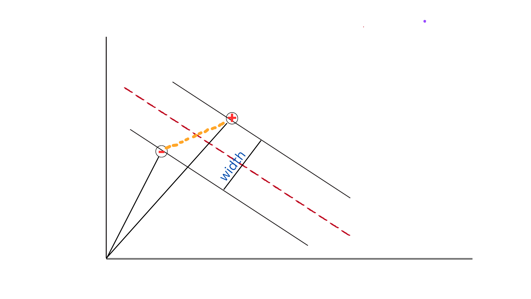
Okay, Now we have a w normal vector which is perpendicular to the decision boundary. Also two support vectors x⁺ and x^- that helps to determine the width of the street.

So the width of the street can be written as follows.

width = (x⁺ - x^- ) • w / ||w||

This is the scaler projection of (x⁺ - x^- ) onto w. Here we are not interested in the vector projection since we need only the length. If you really want to know about scaler projection and the vector projections of the vectors, please refer to this video below.

- YouTube

Bekijk je favoriete video’s, luister naar de muziek die je leuk vindt, upload originele content en deel alles met vrienden, familie en anderen op YouTube.

YouTube

width = (wx⁺ - wx^- ) / ||w|| -———> equation 2

from the equation 1,

• For the positive samples (where y⁺ = +1 ):
  y⁺ × (w^Tx⁺+b) = 1
  +1 × (w^Tx⁺+b) = 1
  w^Tx⁺ = 1-b
• For the negative samples (where y^- = -1):
  y⁺ × (w^Tx⁺+b) = 1
  -1 × (w^Tx⁺+b) = 1
  w^Tx⁺ = -1-b

So, from the equation 2,
width = [ (1-b )- (-1-b)] / ||w|| = 2 / ||w||

Now we have our objective function 2 / ||w|| to be maximized for getting the maximum margin between class boundaries. Instead of maximizing it, we can minimize the ||w|| as well. So we can define our objective function f(w):

f(w) = (1/2 ) • ||w||²

1/2 is just for simplifying the calculations. Now we can minimize the objective function with the constraint: y_i(wx_i+b) = 1 for the support vectors.

y_i(wx_i+b) - 1 = 0

Using the Lagrange theorem, we can minimize f(w) with the given constraint y_i(wx_i+b) - 1 = 0. If L is the width between the boundaries:

L(w,b,α) = 1/2 •||w||² - Σ α_i (y_i(wx + b) -1)

After minimizing this, we can have a weight vector w and the bias b. Then by substituting it to wx + b = 0, we can have the decision boundary of the SVM.

Okay, I hope you understand the concepts and will write another article with many more details about SVMs. If you have got something valuable from this blog post, subscribe to me for articles.