How Weight Initialization Affects Neural Network Performance?

Chanaka Prasanna

28 Mar 2025 • 9 min read

In this blog, we will explore what weight initialization is, why it matters, and how different methods can dramatically impact your neural network's accuracy using PyTorch.

If you do not know about neural networks, I recommend that you go through this article.

Let's imagine a scenario where you might have experienced situations in which a model doesn't perform well or struggles to learn effectively. Sometimes, the issue could be something related to the initialization of your network. Weight initialization is a fundamental yet often overlooked aspect of training neural networks.

What is Weight Initialization?

Do you know how neural networks store the knowledge they obtain during learning? Well, this is where the weights come into play. When you build a neural network, each neuron connection has a weight, which is a numeric value that the network adjusts during training to learn patterns. Weight initialization means assigning these initial numeric values before training begins. Poor initialization can cause slow learning or even stop the network from learning altogether.

Why Does Initialization Matter?

At the start, we have to initialize the weights on the neural network, and then the network will adjust the weights itself based on the training data. These initial values directly affect the accuracy of the model because of the gradient descent algorithm on the neural networks. Gradient descent updates the neural network weights by moving them in the direction of steepest descent, based on computed gradients. The initial values of these weights determine

Starting Point in the Loss Landscape

Poor initialization might place the weights in areas where the gradients are either very large (exploding) or extremely small (vanishing). This negatively affects the early learning stages.

Convergence Speed and Stability

Good initialization methods (e.g., Xavier or He initialization) position the network in favorable regions of the loss landscape, allowing gradient descent to quickly converge toward the optimal minima.

EIt should not have happened.

Because gradient descent directly impacts how quickly and effectively the model learns, the choice of initialization method directly influences the final accuracy and generalization capabilities of your model.

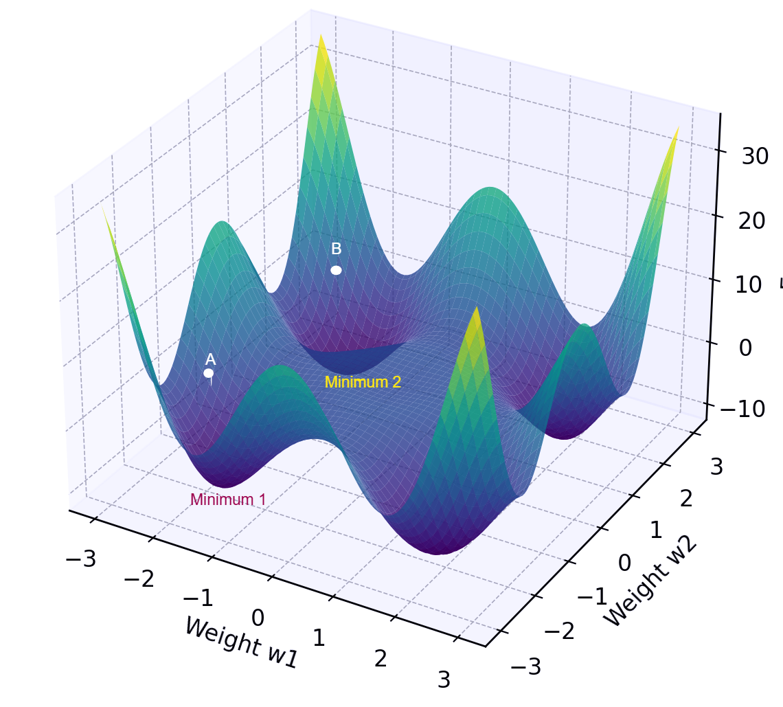
Figure 1 shows a 3D error surface with two initial starting points, A and B.

This table shows the most probable minimums each point may reach

Point	Minimum (Most Probable)
A	Minimum 1
B	Minimum 2

Now, it is clear that, weight initialization directly affects to the accuracy of the model.

Let's talk about the weight initialization techniques using a coding example. So that you can see the effect on the accuracy of each method. The digits dataset (a common dataset in machine learning with images of handwritten digits) will be used.

Setting Up the Experiment

We'll use the digits dataset from scikit-learn. This dataset contains 1797 images of handwritten digits from 0 to 9, each represented as a set of pixel values.

Download full notebook here ⬇️

Let's import all necessary modules here.

import torch
import torch.nn as nn
import torch.nn.functional as F
import numpy as np
from sklearn.datasets import load_digits
from sklearn.model_selection import train_test_split
from sklearn.preprocessing import StandardScaler
from sklearn.metrics import accuracy_score

Let's define a function to set seed values

def set_seed(seed=42):
    torch.manual_seed(seed)
    np.random.seed(seed)
    random.seed(seed)
    if torch.cuda.is_available():
        torch.cuda.manual_seed_all(seed)

set_seed()

Why do we set seeds?

1. Reproducibility

Neural networks training involves random initialization of weights, random shuffling of data, and stochastic optimization (like stochastic gradient descent).
Without setting seeds, results change every run.
Setting a seed guarantees that the same code produces identical results each time, important for debugging, validating results, and comparing models.

2. Fair Comparison of Experiments

When evaluating hyperparameters or different model architectures, random variability makes comparisons unreliable.
Seed ensures every experiment starts identically, isolating the effect of your changes.

Now it's time to load the dataset.

# Load Digits dataset (1797 samples, 64 features)
digits = load_digits()
X = digits.data
y = digits.target

Scale the features

# Standardize the dataset
scaler = StandardScaler()
X = scaler.fit_transform(X)

Split the dataset into a training (80% of the data) and a test (20% of the data) set.

# Train-Test split
X_train, X_test, y_train, y_test = train_test_split(
    X, y, test_size=0.2, random_state=42
)

Convert data into to tensors.

X_train = torch.tensor(X_train, dtype=torch.float32)
y_train = torch.tensor(y_train, dtype=torch.long)
X_test = torch.tensor(X_test, dtype=torch.float32)
y_test = torch.tensor(y_test, dtype=torch.long)

Now, we are going to define our model architecture with 3 layers

# Define the neural network
class DigitNN(nn.Module):
    def __init__(self):
        super(DigitNN, self).__init__()
        self.fc1 = nn.Linear(64, 128)
        self.fc2 = nn.Linear(128, 64)
        self.fc3 = nn.Linear(64, 10)

    def forward(self, x):
        x = F.relu(self.fc1(x))
        x = F.relu(self.fc2(x))
        x = self.fc3(x)
        return x

This neural network (DigitNN) consists of 3 layers:

First layer (fc1): Input size of 64 and output size of 128.
Second layer (fc2): Input size of 128 and output size of 64.
Third layer (fc3): Input size of 64 and output size of 10.

All layers are fully connected (linear) layers.

The forward function dictates exactly how data flows through your neural network, determining the computations performed at each layer and the sequence of transformations the input undergoes to produce the final prediction.

Input (x)

This is the data (numerical input) that enters the neural network.

Hidden Layer 1 (self.fc1)

The input is processed through the first fully connected layer.
F.relu applies the Rectified Linear Unit activation function, introducing non-linearity and helping the model learn complex patterns.

Hidden Layer 2 (self.fc2)

The output from the previous layer becomes input here, again processed by another linear transformation and ReLU activation.

Output Layer (self.fc3)

The final fully connected layer outputs predictions.
No activation function here usually means this model outputs raw scores (logits), which are typically passed to a loss function like CrossEntropyLoss, which internally applies softmax.

Then we are gonna define a function to train and evaluate the models, because we have to train and evaluate models several times for each technique.


def train_and_evaluate(model):
    criterion = nn.CrossEntropyLoss()
    optimizer = torch.optim.Adam(model.parameters(), lr=0.005)

    model.train()
    for epoch in range(100):
        optimizer.zero_grad()
        outputs = model(X_train)
        loss = criterion(outputs, y_train)
        loss.backward()
        optimizer.step()

    model.eval()
    with torch.no_grad():
        predictions = model(X_test).argmax(dim=1).numpy()
        accuracy = accuracy_score(y_test, predictions)
    
    return accuracy

The train_and_evaluate function trains the provided neural network (DigitNN) and evaluates its accuracy on unseen data. It uses Cross-Entropy Loss to measure prediction errors and the Adam optimizer (with a learning rate of 0.005) to optimize model weights. The model undergoes training for 100 epochs, repeatedly updating its parameters to minimize the loss. After training, the function evaluates the model on the test dataset, computing the accuracy by comparing predicted labels against true labels. Finally, it returns this accuracy as an indicator of the model’s performance.

Now, we are going to try some weight initialization techniques. Then we can compare the results from each technique.

Zero Initialization

If we set all weights to zero, every neuron learns the same feature by making all identical. This symmetry prevents effective learning.

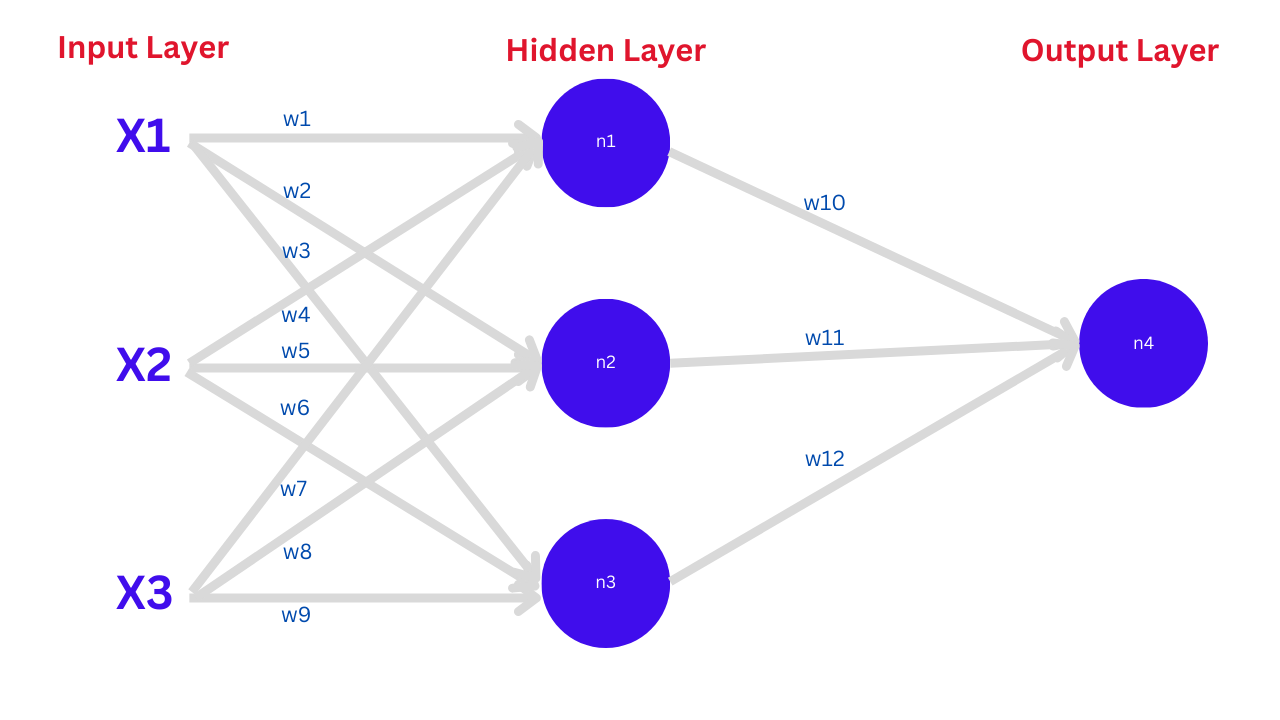
For simplicity, let's forget about the bias of the neurons. Then the induced local field at each neuron of the hidden layer

Also, the outputs from neurons n1 , n2 , n3 and n4 are f1 , f2 , f3 and f

If all weights in a neural network are initialized to zero and the activation function for all layers is ReLU, here’s what happens:

Forward Pass Calculation (for neuron n1 )

Each neuron’s output is calculated as z
z = Σ w_i x_i + b
Since all weights (w) are initialized to 0, we get
z = 0 * x₁ +0 * x₂ + 0 * x₃ + b = b
Assuming bias (b) is also initialized to 0, then
z = 0

ReLU Activation

The ReLU function is defined as:
g(z) = max(0, z)
It outputs the input directly if it's positive, and zero otherwise
Since ( z = 0 ), applying ReLU
f1 = g(0) = 0
Similarly, the hidden layer outputs (f1, f2, f3) will all be 0. That means all neurons have learned the same features. It should not have happened.

Propagation to Output Layer

The same process repeats for the output layer:
z_output = w₁₀f₁ + w₁₁f₂ + w₁₂f₃ + b = 0 (assuming the bias b as zero)
Since f1,f2,f3, and weights are zero, the output of the neuron n4 is also 0.

Final Result

All neurons will output 0, regardless of input values.
This results in a dead network, meaning it cannot learn any patterns.

Here is the code for zero-weight initialization.

model_zero = DigitNN()

# Zero initialization
for param in model_zero.parameters():
    nn.init.constant_(param, 0.0)

acc_zero = train_and_evaluate(model_zero)
print(f"Accuracy with Zero Initialization: {acc_zero * 100:.2f}%")

This is the accuracy we have got.

Typically, accuracy will be very poor, around 10%, since the network struggles to break symmetry.

Random Initialization

Higher random weight values(Ex:2,3,6) generated from a normal distribution

When we give initial values to the weights, we are embedding some unknown knowledge into the network. If those values are higher, then the network needs to unlearn the unknown knowledge first and then relearn. So it takes time and will have low accuracy. And this will cause the exploding gradient problem as well.

This is the code for the experiment. Here we generate initial weights around 5

model_high = DigitNN()
set_seed()

# High-value random initialization (mean=5, std=3)
for param in model_high.parameters():
    nn.init.normal_(param, mean=5.0, std=3.0)

acc_high = train_and_evaluate(model_high)
print(f"Accuracy with High-Value Initialization: {acc_high * 100:.2f}%")

This is the accuracy we have got.

Usually, you'll see very low accuracy due to unstable gradients.

Lower random weight values(Ex:0.2,0.05,0.4) generated from a normal distribution

To solve the above problem, we can initialize weights with very small values.

This is the code for the experiment. Here we generate initial weights around 0.2

model_low = DigitNN()
set_seed()

# Low-value random initialization (mean=0.2, std=0.05)
for param in model_low.parameters():
    nn.init.normal_(param, mean=0.2, std=0.05)

acc_low = train_and_evaluate(model_low)
print(f"Accuracy with Low-Value Initialization: {acc_low * 100:.2f}%")

This is the accuracy we have got.

Accuracy often jumps significantly, showing stable training. But sometimes, smaller gradients may cause a vanishing gradient problem.

To enhance accuracy further and avoid the vanishing and exploding gradient problem, we have to pay attention to the activation function as well. So we can do weight initialization by focusing on the activation functions by using the He and Xavier weights initialization techniques.

He Initialization (Kaiming)

He initialization is specifically designed for neural networks using ReLU activations.

model_he = DigitNN()
set_seed()

# He initialization
for name, param in model_he.named_parameters():
    if 'weight' in name:
        nn.init.kaiming_normal_(param, nonlinearity='relu')
    elif 'bias' in name:
        nn.init.constant_(param, 0.0)

acc_he = train_and_evaluate(model_he)
print(f"Accuracy with He Initialization: {acc_he * 100:.2f}%")

This is the accuracy we have got.

Typically gives excellent results, thanks to effective gradient flow.

Xavier Initialization

Xavier initialization is specifically designed for neural networks using tanh and sigmoid activations.

model_xavier = DigitNN()
set_seed()

# Xavier initialization
for name, param in model_xavier.named_parameters():
    if 'weight' in name:
        nn.init.xavier_normal_(param)
    elif 'bias' in name:
        nn.init.constant_(param, 0.0)

acc_xavier = train_and_evaluate(model_xavier)
print(f"Accuracy with Xavier Initialization: {acc_xavier * 100:.2f}%")

This is the accuracy we have got.

Xavier initialization often provides accuracy similar to He initialization.

Conclusion

Through these experiments, we've clearly seen how weight initialization methods drastically affect the accuracy of a neural network. Zero or inappropriate initialization can hinder learning significantly. Proper initialization like He or Xavier ensures stable gradients, faster convergence, and higher accuracy.

Using PyTorch makes experimenting straightforward, allowing quick testing and iteration. Remember, while hyperparameters and model architecture are essential, always begin your neural network journey with proper weight initialization for optimal results!