How to Handle Class Imbalance in Your Dataset

Class imbalance occurs frequently in real-world datasets. But what exactly is class imbalance? Let’s consider an example. Suppose we are dealing with a dataset to predict whether a given patient has cancer or not. Typically, most people do not have cancer, but a small number may have it. For instance, in a group of 1000 patients, about 50 might have cancer. This creates a class imbalance because one class has around 950 patients, while the other has about 50 patients, leading to a bias towards the majority class.

Other examples of imbalanced datasets in the real world include

• Fraud Detection - In financial datasets, fraudulent transactions are much rarer compared to non-fraudulent ones. For example, only 1 in 1000 transactions might be fraudulent.
• Spam Detection — In email datasets, the number of spam emails is typically much lower compared to legitimate emails. For instance, out of 1000 emails, only about 100 might be spam.
• Disease Outbreaks - In medical datasets, certain diseases are very rare compared to others. For example, in a dataset tracking various diseases, rare diseases might make up only a tiny fraction of the total cases.
• Customer Churn - In business datasets, the number of customers who cancel their subscription (churn) is often much smaller compared to those who stay. For example, only 50 out of 1000 customers might churn in a given period.

These examples illustrate how class imbalance can manifest in various domains, posing challenges for machine learning models that need to be addressed.

How Can We Deal with Class Imbalance?

There are many techniques to address class imbalance. Let’s consider a few of them one by one

Undersampling Majority Class

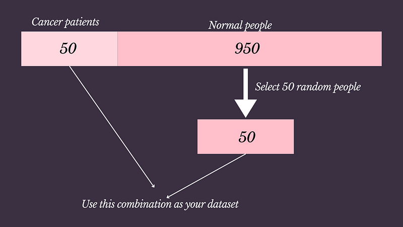
This technique involves reducing the number of instances in the majority class to match the number of instances in the minority class. While this can help balance the classes, it may lead to the loss of important information from the majority class because we will lose the data from the majority class.

Oversampling Minority Class(Blind Copy)

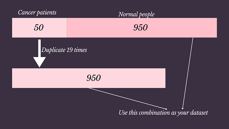
Oversampling involves increasing the number of instances in the minority class by duplicating existing instances. This helps balance the classes but can lead to overfitting, as the model might learn to memorize the duplicated instances.

Oversampling minority class using SMOTE

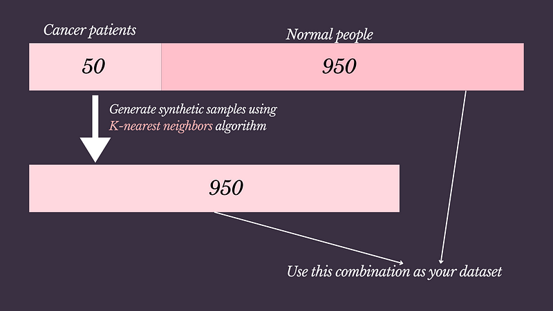
SMOTE (Synthetic Minority Over-sampling Technique) generates synthetic instances of the minority class by interpolating between existing instances. It uses the K-nearest neighbors algorithm to generate data. It helps create a more diverse set of instances for the minority class, reducing the risk of overfitting compared to blind copy oversampling.

Ensemble Methods

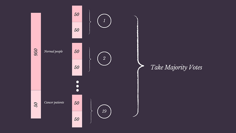
Ensemble methods combine the predictions of multiple models to improve performance. Techniques like bagging and boosting can be particularly effective for dealing with class imbalance, as they can reduce the impact of the majority class dominating the predictions.

In this given example, we divide 950 people into 19 samples. Then each sample has 50 records. Then combine each sample with the cancer patient sample. Now we can use these combinations with models and take the majority of results as output

Let’s see these techniques in action

Introduction to the Dataset

In this blog post, I will be using a dataset of credit card transactions made by European cardholders in September 2013. This dataset is used to detect fraudulent transactions to ensure customers are not wrongly charged for items they did not purchase.

The dataset includes transactions over two days, with 492 frauds out of 284,807 transactions, making it highly unbalanced as frauds account for only 0.172% of all transactions. All features in the dataset are numerical, but their original names are not given due to confidentiality reasons. Instead, they are labeled as V1, V2, …, V28, which are the principal components obtained through PCA transformation. Additionally, there are two features, ‘Time’ and ‘Amount’, which have not been transformed by PCA. ‘Time’ represents the seconds elapsed since the first transaction, and ‘Amount’ is the transaction amount. The response variable ‘Class’ is 1 for fraud and 0 for non-fraud.

Link for the dataset -https://www.kaggle.com/datasets/mlg-ulb/creditcardfraud/data

Link For Notebook — https://github.com/Chanaka-Prasanna/Datasets/blob/main/class-imbalence/class_imbalence.ipynb

Import necessary tools

import pandas as pd 
import numpy as np 
from sklearn.model_selection import train_test_split 
from sklearn.linear_model import LogisticRegression 
from sklearn.metrics import classification_report

Import the dataset.

df = pd.read_csv('creditcard.csv') 
df.head()

Tran the model and get the classification report

#Split the dataset  
X = df.drop('Class',axis=1) 
y = df['Class'] 
 
# Split the dataset into training and testing sets 
X_train, X_test, y_train, y_test = train_test_split(X, y, test_size=0.2, random_state=42)

Lets define a function to train our model and print classification report

# Function to train the model and print classification report 
def train_model(X_train, X_test, y_train, y_test): 
    # Train a logistic regression model 
    model = LogisticRegression(max_iter=1000) 
    model.fit(X_train, y_train) 
     
    # Make predictions 
    y_pred = model.predict(X_test) 
     
    # Generate classification report 
    report = classification_report(y_test, y_pred, zero_division=0) 
    print(report)

train_model(X_train, X_test, y_train, y_test)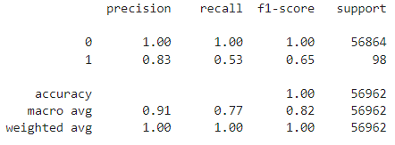

Here look at the f1 score. There is no balence in those two classes

Let’s use the above-mentioned techniques to solve this problem.

Undersampling Majority Class

Let's see the shape of our data

#Shape of our data 
class_0 = df[df['Class'] == 0] 
class_1 = df[df['Class'] == 1] 
class_0.shape, class_1.shape 
 
# Result -> ((284315, 31), (492, 31))

This is a highly imbalanced dataset.

Now, we can randomly select the sample of 492 records from the majority class

# Randomly select the sample of 492 records from majority class 
class_0_sample = class_0.sample(492) 
class_0_sample.shape 
 
# Result -> (492, 31)

Concatenate the new sample of class 0 and class 1

new_df = pd.concat([class_0_sample,class_1],axis=0) 
new_df.shape 
 
# Result -> (984, 31)

Splitting the dataset

# Split the dataset into features and target variable 
X = new_df.drop('Class',axis=1) 
y = new_df['Class'] 
 
# Split the dataset into training and testing sets 
X_train, X_test, y_train, y_test = train_test_split(X, y, test_size=0.2, random_state=42,stratify=y)

Train the model and print the classification report using a predefined function

train_model(X_train, X_test, y_train, y_test)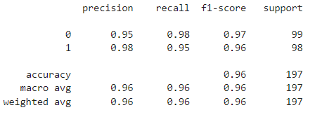

Now the precision scores are high and balanced for both classes. But remember, here we have some information loss. That is not good for the predictions.

Oversampling the minority class

#Shape of our data 
class_0 = df[df['Class'] == 0] 
class_1 = df[df['Class'] == 1] 
class_0.shape, class_1.shape 
 
# Result -> ((284315, 31), (492, 31))

Now, Let's create a sample with 284315 records in class 1. Currently we have 492 records and we use the same records to create a new sample. Remember you need to add replace = True. The parameter replace=True in the sample() function allows for sampling with replacement. This means that the same record can be selected more than once.

# Randomly select the sample of 284315 records from minority class 
class_1_sample = class_1.sample(284315,replace=True) 
class_1_sample.shape 
 
# Result -> (284315, 31)

Now, Let’s concatenate a new sample of class 1 and class 0.

#Combine the data from class 0 and class 1 
new_df = pd.concat([class_0,class_1_sample],axis=0) 
new_df.shape 
 
# Result -> (568630, 31)

# Split the dataset into features and target variable 
X = new_df.drop('Class',axis=1) 
y = new_df['Class'] 
 
# Split the dataset into training and testing sets 
X_train, X_test, y_train, y_test = train_test_split(X, y, test_size=0.2, random_state=42,stratify=y)

# Train the model and print classification report 
train_model(X_train, X_test, y_train, y_test)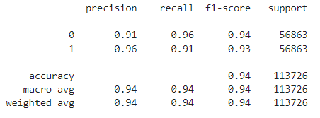

You can see, now also we can have high and balanced f1-scores.

SMOTE Method

# Split the dataset into features and target variable 
X = df.drop('Class',axis=1) 
y = df['Class']

Now we need to install below package for apply SMOTE method

#Install necessary packages 
!pip install imbalanced-learn

#Import SMOTE and create a instance 
from imblearn.over_sampling import SMOTE 
smote = SMOTE(sampling_strategy='minority')

sampling_strategy='minority' — This parameter specifies the resampling strategy. By setting it to 'minority', SMOTE will generate synthetic samples only for the minority class to balance it with the majority class.

y.value_counts() # Check the existing value counts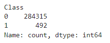

Let's create new datasets using SMOTE technique

#Create records for monority class using SMOTE 
X_sample, y_sample = smote.fit_resample(X,y) 
y_sample.value_counts()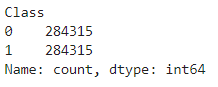

Now we have a balanced dataset for both classes.

# Split the dataset into training and testing sets 
X_train, X_test, y_train, y_test = train_test_split(X_sample, y_sample, test_size=0.2, random_state=42,stratify=y_sample) 
y_train.value_counts(),y_test.value_counts()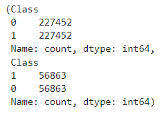

# Train the model and print the classification report 
train_model(X_train, X_test, y_train, y_test)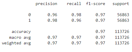

Hmmmm… So far the highest f1-score right? Till now, we can say this is the best method since we use the k-nearest neighbors algorithm to create synthetic data rather than duplicating or selecting existing data.

Using Ensemble method

Here we are using RandomForestClassifier which is one of the models that uses the ensemble method.

# Split the dataset into features and target variable 
X = df.drop('Class',axis=1) 
y = df['Class'] 
 
# Split the dataset into training and testing sets 
X_train, X_test, y_train, y_test = train_test_split(X, y, test_size=0.2, random_state=42,stratify=y) 
y_train.value_counts()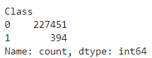

from sklearn.ensemble import RandomForestClassifier 
 
mdl =  RandomForestClassifier(random_state=42) 
mdl.fit(X_train,y_train) 
y_preds = mdl.predict(X_test) 
print(classification_report(y_test,y_preds))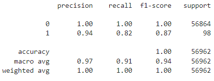

In this case, since we used the Random Forest algorithm, we did not need to resample the dataset. However, the given results suggest that the model may be overfitting. This overfitting could be due to the characteristics of the Random Forest algorithm itself. Therefore, further investigations are required, including hyperparameter tuning.

Handling class imbalance is crucial for improving the performance of machine learning models. This blog post covered four techniques to address class imbalance: undersampling the majority class, oversampling the minority class, using SMOTE, and employing ensemble methods. Through practical examples with a credit card fraud detection dataset, we demonstrated the strengths and weaknesses of each approach. While undersampling and oversampling are straightforward, they can lead to information loss and overfitting, respectively. SMOTE, which creates synthetic samples, provided the most balanced results in this case. Ensemble methods, like Random Forest, can handle imbalance without resampling but may require careful tuning to avoid overfitting. Choosing the right technique depends on the specific dataset and problem, but SMOTE and ensemble methods often offer robust solutions.

If you found this useful, follow me for future articles. It motivates me to write more for you.

Follow me on Medium

Follow me on LinkedIn