Learning

Evaluating Model Performance with K-Fold Cross-Validation - A Practical Example

Chanaka Prasanna

Jul 31, 2024 • 6 min read

In the previous article, I explained cross-validation. Now, I’m going to show you K-fold cross-validation in action. This is one of the most common techniques in cross-validation. Remember, if your dataset is imbalanced, you should first address this issue before using any cross-validation technique.

K-fold cross-validation involves splitting your dataset into K parts (folds). Then, the technique uses one fold to test the model and the remaining K-1 folds to train the model. Each fold acts as a test set in turn, during K iterations.

You can download the notebook here.

In this example, I’m using the California Housing dataset from scikit-learn. Since we need to predict housing prices, this is a regression problem. Therefore, I’ll use the RandomForestRegressor as the model (estimator).

Let’s dive into the code now

Import necessary tools

from sklearn.datasets import fetch_california_housing
from sklearn.ensemble import RandomForestRegressor
from sklearn.model_selection import train_test_split,cross_val_score
from sklearn.metrics import r2_score,mean_absolute_error,mean_squared_error
import numpy as np
import pandas as pd

Fetch data

housing = fetch_california_housing()
housing

housing_df = pd.DataFrame(housing['data'],columns = housing['feature_names'])
housing_df['target'] = housing['target']
housing_df.head()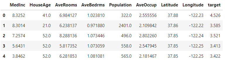

This code segment fetches the California Housing dataset and stores it in a variable called housing. It then creates a pandas DataFrame from the dataset, using the feature names as column labels for the data. Next, it adds a new column to the DataFrame for the target values (housing prices). Finally, the code displays the first few rows of the DataFrame to provide a preview of the data.

np.random.seed(42)

X = housing_df.drop('target',axis=1)
y = housing_df['target']

X_train,X_test, y_train,y_test = train_test_split(X,y,test_size = 0.2)


mdl = RandomForestRegressor()
mdl.fit(X_train,y_train)

This code sets a random seed for reproducibility, then prepares the data by separating features (X) from the target values (y). It splits the data into training and testing sets, with 20% of the data reserved for testing. Finally, it initializes a Random Forest Regressor model and trains it using the training data.

Regression Model Evaluation Metrics

Link - https://scikit-learn.org/stable/modules/model_evaluation.html#regression-metrics

The ones we are going to cover are:

R^2 (Pronounced r-squared) or coefficient of determination
Mean absolute error (MAE)
Mean squared error (MSE)

Now, Let's consider these values without cross-validation

R2 Score

The R² score measures how well a model's predictions match the actual data. It compares the model's predictions to the average of the actual target values. The score ranges from negative infinity to 1: a score of 1 means perfect predictions, while a score of 0 means the model's predictions are no better than simply using the average of the target values.

y_preds =  mdl.predict(X_test)
r2_score(y_true=y_test,y_pred=y_preds)

# output => 0.8066196804802649

Mean Absolute Error (MAE)

The Mean Absolute Error (MAE) measures the average of the absolute differences between the predicted values and the actual values. It tells you how far off your model’s predictions are from the true values, providing a straightforward measure of prediction accuracy.

Data and MAE are on same scale

# MAE 

y_preds = mdl.predict(X_test)
mae = mean_absolute_error(y_test,y_preds)

mae

# output => 0.3265721842781009

Mean Squared Error (MSE)

The Mean Squared Error (MSE) calculates the average of the squared differences between the predicted values and the actual values. Because MSE squares the errors, it penalizes larger errors more heavily. To get back to the original scale of the data, you can use the Root Mean Squared Error (RMSE), which is the square root of the MSE.

# MSE


y_preds = mdl.predict(X_test)
mse = mean_squared_error(y_test,y_preds)
mse

# output => 0.2534678520824551

Now, we are going to calculate the same metrics using cross-validation

Refer to this table for choosing scoring parameters . According to the problem you are solving (Classification, Regression, or Clustering), the scoring parameters are different. Go through the link and find those.

R2 score (using cross-validation)

np.random.seed(42)

cv_score =  cross_val_score(mdl,X,y,cv=5,scoring=None), # If scoring is            
# None,Model's default scoring evaluation metric is used. (in our case, it is r2  # score)

# Take the mean
np.mean(cv_score)

# output => 0.6521420895559876

In this case, we used scoring='None', which means the default metric used is the R² score. We can verify this by comparing it with the code segment below, as both segments will yield the same values.

np.random.seed(42)
r2 =  cross_val_score(mdl,X,y,cv=5,scoring='r2')
r2
# output => (array([0.51682354, 0.70280719, 0.74200859, 0.61659773, 0.68247339]),)

np.mean(r2)

# output => 0.6521420895559876

The cross_val_score function performs 5-fold cross-validation on the regression model (mdl) using the R² score as the metric (scoring='r2'). This means the dataset is split into 5 parts (cv=5), with each part serving as the test set once while the remaining 4 parts are used for training.

The function cross_val_score returns an array of R² scores, one for each fold. In this example, the R² scores for the 5 folds are approximately [0.5168, 0.7028, 0.7420, 0.6166, 0.6825]. The np.mean(r2) calculates the average of these scores, which is about 0.6521.

This average R² score gives a more comprehensive view of the model's performance across different subsets of the data compared to a single R² score obtained from one test/train split.

MAE (using cross-validation)

np.random.seed(42)
mae =  cross_val_score(mdl,X,y,cv=5,scoring='neg_mean_absolute_error')
mae

# output => array([-0.54255936, -0.40903449, -0.43716367, -0.46911343, -0.47319069])

np.mean(mae)

# output => -0.4662123287693799

In this code, the cross_val_score function performs 5-fold cross-validation (cv=5) on the model using Mean Absolute Error (MAE) as the scoring metric (scoring='neg_mean_absolute_error').

Since scoring='neg_mean_absolute_error' returns negative values you may be wondering. Let's clarify it.

MAE measures the average absolute difference between predicted and actual values. Lower MAE values indicate better model performance because fewer errors mean better predictions.

Since cross_val_score is designed to maximize scores, it’s set up to prefer higher values. To adapt MAE, which benefits from being lower, the function returns the negative of the MAE. For example, if the MAE is 5, it returns -5; if the MAE is 9, it returns -9.

This sign flip allows the function to follow its maximization convention. A higher negative value (less negative) corresponds to a smaller MAE, which indicates better performance. Thus, -5 is better than -9 because -5 (less negative) represents a lower MAE, reflecting fewer errors and better predictions.

I hope you got the idea. Let's continue from where we left.

The np.mean(mae) function calculates the average of these negative MAE scores, resulting in approximately -0.4662. This average provides an overall measure of the model's prediction accuracy across different data subsets. To get the actual MAE, you would take the negative of this value.

MSE (using cross-validation)

np.random.seed(42)
mse =  cross_val_score(mdl,X,y,cv=5,scoring='neg_mean_squared_error')
mse

# output => array([-0.51906307, -0.34788294, -0.37112854, -0.44980156, -0.4626866 ])

np.mean(mse)

# output => -0.43011254261460774

In this code, cross_val_score evaluates the regression model's performance using 5-fold cross-validation (cv=5) with the Mean Squared Error (MSE) as the metric. The scoring='neg_mean_squared_error' parameter indicates that the function returns negative MSE values, as minimizing MSE is equivalent to maximizing the negative MSE.

The output array contains negative MSE values for each fold: [-0.5191, -0.3479, -0.3711, -0.4498, -0.4627]. The average of these negative MSE values, calculated as np.mean(mse), is approximately -0.4301. This average negative MSE represents the typical squared error of the model's predictions across different data subsets, with the actual MSE being around 0.4301.

Cross-validation, especially with k-fold (like 5-fold), provides a more reliable evaluation of a model’s performance compared to a single train-test split. It helps in understanding how well the model generalizes to different subsets of the data. When using a model like RandomForestRegressor, cross-validation helps mitigate the risk of overfitting and provides a more robust estimate of performance. This approach ensures that the evaluation is less dependent on the particular train-test split and gives a more comprehensive view of the model’s effectiveness across various data splits.

If you found this article helpful, subscribe to me for more like this. Also, make sure you follow me on LinkedIn.